Review the Policies and Strategies of Export and Import Practices in Ethiopia

Introduction

Ethiopia is an E African country with a population of near 105 million (Key Intelligence Agency, 2015; Primal Statistical Agency of Federal democratic republic of ethiopia, 2016) and a GDP of 72 billion U.s.a. dollars (Central Intelligence Agency, 2015). Over 70% of the labor force depends on agriculture for their livelihood (Key Intelligence Agency, 2015) and agriculture contributes to about 40% of the Gdp of the country (Central Intelligence Agency, 2015). Moreover, almost 60% of all Ethiopia'due south exports are generated from the agronomical sector (MIT, 2018). Notwithstanding, agriculture in Ethiopia is characterized by smallholder forming and is extremely sensitive to weather and climate variation. The contempo 2015 and 2017 El Nino event, for example, led to drought across much of the country. Resulting crop and livestock losses led the government of Ethiopia to telephone call for emergency aid to over eighteen million people, via a combination of domestic and international relief efforts (USAID, 2016). These impacts are consequent with Ethiopia'southward past sensitivity to climate shocks, which has motivated a number of studies on the agricultural impacts of climate variability in Ethiopia (Mccornick et al., 2008; Di Falco and Veronesi, 2012; Iizumi et al., 2014; Bakker et al., 2018) and other detailed strategies to combat food shortage (Wossen et al., 2016; Di Falco and Zoupanidou, 2017).

In improver to climatic shocks, the country'southward agriculture and food supply chain is not immune to other exogenous shocks. The 2008 global financial crises, which caused a worldwide food price hike, brought Ethiopian agronomical commodities into deep distress. Researchers deployed surveys to quantify the impact of the price hike in terms of changes in nutrient consumption patterns and changes in food intake (Alem and Söderbom, 2012; Kumar and Quisumbing, 2013). The agin effect of such a global result motivated the Ethiopian authorities to implement an export ban on nutrient grains, including teff, indefinitely.

Teff is a critical grain for Federal democratic republic of ethiopia. It is central to Ethiopian diets equally it is the primary and preferred ingredient in Ethiopian bread (injera), and information technology has as well shown significant potential since it is unique, has high nutrient content and is gluten free (Minten et al., 2018). The main goal of the export ban policy was to limit the upward pressure on domestic grain prices. A study analyzed the impacts of the ban on the country's macroeconomy under export ban policy scenarios (Woldie and Siddig, 2009). While predicting that the policy volition indeed fulfill its goal of reducing domestic food prices, the study found that it comes at a cost of social welfare, quantified postal service facto at about $148 million. The government export ban policy was also studied extensively in Sharma (2011). In this study, the regime'south export ban policy was compared to like policies in other countries and was criticized equally a poorly designed restrictive measure. As a outcome, the authors propose an culling policy package for the government, including various taxation regimes, price floors for exports, and government to government sales, amongst others. The study did non, nevertheless, perform an assay of the welfare impacts of potential alternative policies.

While the existing literature quantifies the effects of global food prices and governmental policies on agronomical food commodities, to the best of our knowledge, there are few models that can analyze the distributed impacts of future policy changes across disaggregated regions under different policy scenarios. In that location are some mature partial-equilibrium models that can exist used to understand the impact of agricultural policies at land scale, including the International Model for Policy Analysis for Agricultural Commodities and Trade (IMPACT) (Rosegrant et al., 2008; Robinson et al., 2015), rice outlook model (Wailes and Chavez, 2011) and globe food model of agriculture (FAO, 1998), but these tools do not provide sub-national assay in Ethiopia and about other small to mid-size countries. Farther, a detailed assay of the upstream, midstream and downstream domestic supply concatenation of teff, including celebrated variation in production, sensitivity of product, transportation and consumption and welfare effects is available from IFPRI (Minten et al., 2018).

In this newspaper, nosotros accost the directly impacts in regional teff markets, transport patterns, and market actors' profits beyond disaggregated regions in Ethiopia due to changes in the teff export ban policy. The specific focus on teff is motivated by the fact that teff has been predicted by researchers to become a new super-ingather (Provost and Jobson, 2014; Crymes, 2015), with dramatically increased international demand. Our assay complements the existing macroeconomic analyses (Woldie and Siddig, 2009; Sharma, 2011) in providing a detailed understanding of the regional furnishings of such policy changes within Ethiopia, along with comparing the effects of the policy change under potential shifts in the global need curve.

Specifically, we address the following questions regarding potential relaxation or removal of teff export restrictions:

1. How practise regional microeconomic market indicators change under different teff merchandise policy scenarios?

two. Which regions in the country are afflicted the nearly by a change in the teff export ban policy?

3. Which regional market actors are affected the near by a modify in the teff export ban policy?

To answer these questions, we present an advanced integrated partial-equilibrium model, chosen the Distributed Extendible COmplementarity model (DECO). The model is an extension of the original DECO model introduced in Bakker et al. (2018) to model food systems. The model is a partial equilibrium model that represents the determination of multiple market actors, non-cooperatively maximizing their objective (typically profit or utility) with a detailed representation of the agro-economic properties of the regions in the land and the food markets therein. This detailed modeling enables us to present the regionalized effects of policy changes to the country'southward food markets. To distinguish this version of the model from that in Bakker et al. (2018), we refer to information technology equally DECO2. In detail, the specific contributions of this paper in terms of modeling are:

ane) Updating the production regions to coincide with government defined agro-climatic "adaptation zones" (Figure i), equally opposed to authoritative regions in the original model. This allows u.s. to correspond product activities integrated with climate and soil characteristics, rather than arbitrary administrative regions.

2) Endogenously modeling transportation in the country by splitting the country into Thiessen polygons to account for both inter-regional and intra-regional trade

3) Incorporating more detailed water activities to integrate with climate variability, ingather yield, and hydrological conditions.

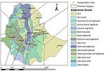
Figure 1. Adaptation zones of Federal democratic republic of ethiopia and regions centered around transportation hubs or nutrient markets. Based on Deribew et al. (2015).

Nosotros apply the updated model to simulate several scenarios of teff export policies that potentially affect teff marketplace dynamics within the country, and nosotros compare the performance of different market actors under each of the scenarios. Such an analysis helps compare policy under diverse stimuli and identify quantifiable differences in regionalized benefits for different market actors such as producers too as consumers. The balance of the paper is divided as follows. Section Model Description describes the features and the enhancements in the DECO2 model. Section Base of operations Instance Calibration and Scenarios presents the scenarios we analyze in particular and explains the methods employed in implementing these scenarios. Section Results contains results and analysis, and department Conclusions and Discussions includes conclusions and an cess of limitations.

Model Description

Partial equilibrium models are useful tools for studying the effect of a policy change or other intervention on certain parts of the market. This arroyo allows one to understand the effect of policy changes at a disaggregated micro level, which is a characteristic of detail involvement when studying nutrient systems. DECO2 accordingly is an integrated partial-equilibrium model that is designed to simulate supply chains in the nutrient market in Ethiopia. Since our model is a fractional equilibrium model, we presume that most of the macroeconomic variables (i.due east., population, Gross domestic product) are constant. Modelers follow this arroyo typically to capture more granular detail than general equilibrium models, which factor all macroeconomic variables only do not explicitly model regional markets and infrastructure. Partial-equilibrium models are more than suited for analyzing localized changes under isolated shocks or scenarios, and non for projecting futurity macroeconomic trends. In DECO2, nosotros compute the equilibrium resulting from the interaction of five types of aggregated marketplace actors in the model, namely:

(i) Ingather producers

(ii) Livestock raisers

(iii) Food distribution operators

(iv) Food storage operators or warehouses

(5) Consumers

Each market player competitively maximizes their own objective under the assumption of perfect competition marketplace construction. In the rest of the department, nosotros formally depict the spatial disaggregation and fourth dimension steps used in the model. Then we sequentially draw the role of each marketplace actor in the model.

Spatial Disaggregation

Nosotros use two types of spatial disaggregation in the model, namely disaggregation past accommodation zone to correspond production and consumption, and disaggregation past regions centered with selected transportation hubs to model regional nutrient markets and transportation. From a modeling perspective, however, information technology is inappropriate to use politically delineated areas (for example, the administrative regions) that might non account for crop suitability, productivity, and the diverse Ethiopian climate zones with steep pluvial gradients. Even so, in Ethiopia, 14 adaptation zones separate the country into regions of similar climate patterns and soil fertility patterns, so that in our model, whatsoever crop will have a representative yield beyond a single adaptation zone. These zones take been divers by the government of Ethiopia every bit a framework for climate resilience efforts to boost production by allowing officials to pattern climatically-relevant adaptation strategies at scale, and to place populations that might face up elevated risk under climate change (Deribew et al., 2015), merely given the dominance of smallholder subsistence agriculture in Ethiopia, and the idea that consumption preferences are dictated by what is grown in a detail region, nosotros use the adaptation zones as the unit of measurement for modeling consumption besides.

However, the adaptation zones are not necessarily a face-to-face stretch of state, and they can spread over long distances geographically. For this reason, we cannot employ adaptation zones to model food transport. Therefore, we divide the state into regions surrounding 15 transportation hubs or food markets and assume that all send occurs between pairs of these markets. The markets were chosen to ensure that they were both reasonably spread across the country and correspond to highly populated cities in the state. We use the markets every bit seeds to a Voronoi tessellation (Voronoi, 1908), such that the country is partitioned into Thiessen polygons, each which contains exactly one market (Figure 1). The Thiessen polygons accept the property that the market contained in the polygon is the closest marketplace to every point within the polygon (Voronoi, 1908). We assume that the aggregated crop producer in whatsoever accommodation zone sells in one or more than markets proportionally based on the overlap between the adaptation zone and each marketplace's Thiessen polygon. This indicates that the crop producers sell in the markets closest to them geographically.

Exports from Ethiopia are modeled past adding an external node to the collection of transportation hubs. The prices in the external node are set by global demand and supply for a nutrient commodity. For teff, we draw the international price from (USDA Foreign Agricultural Service, 2013). We do not simulate demand-supply dynamics external to Federal democratic republic of ethiopia, and we also do not consider production outside of Ethiopia, which is a small just growing phenomenon. Any consign from Ethiopia is sent to the external node and any import to Ethiopia comes in through the external node, which is continued to other nodes via the national majuscule, Addis Ababa.

Time Steps

DECO2 solves for equilibrium in semi-almanac time steps, each step corresponding to a cropping flavor. We solve the model on a year-past-yr basis to simulate the responses due to policy changes, without information almost futurity years. 2 additional years are solved in each iteration and then dropped to remove excessive model short-sight. We call this the rolling-horizon process and refer readers to Sethi and Sorger (1991) for a rigorous analysis of the approach.

Within each year, nosotros explicitly model the two cropping seasons of Federal democratic republic of ethiopia. The meher flavour, which relies on the summertime kremt rains (primarily June-September), and the springtime belg flavour, which relies primarily on March-April rains. The meher flavour is the primary cropping flavor, in which more than seventy% of all food is produced.

We now discuss the six market place actors nosotros model in DECO2. They are all profit maximizing market actors, bated from the consumer who maximizes utility. The model assumes a non-cooperative game played between the market actors nether an supposition of perfect competition.

Crop Producers

We presume that the agricultural country in Federal democratic republic of ethiopia is used to produce either master food crops or secondary food crops or greenbacks crops. The primary food crops are teff, sorghum, barley, maize and wheat, the secondary food crops are pulses, vegetables and fruits, and the cash crops are java and oil seeds. The chief crops are grown in about lxx% of the total cropping area while the secondary and greenbacks crops are grown in roughly 20 and 10% of the total cropping area, respectively (Cardinal Statistical Agency of Ethiopia, 2015). Nosotros assume that in that location is a representative aggregate ingather producer in each adaptation zone who always makes a production decision subject to the express farm land available. Factor inputs other than farm land in this model are assumed to be invariant over the menstruation of assay. Appropriately, the aggregate crop producer decides on the size of farm land allotted to each crop with the objective of maximizing profits. In the zone z, for the ingather c, during the cropping season south of year y, the problem of the nutrient producer can be written equally:

$\underset{A_{ZCSY}}{\text{max}}{\displaystyle \sum _{c,s,y}\left({\displaystyle \sum _n{Q}_{zncsy}^{F\to D}{\pi }_{nc\mathrm{south}y}^{D\to F}-C_{zcsy}^F{A}_{zcsy}}\right)}-\text{penalty}\text{terms}$

subject to:

$\begin{array}{lll}{\displaystyle \sum _c}{A}_{zcsy}=A_{z\mathrm{southward}}^{Total}& \left({\delta }_{zsy}^{\mathrm{ane}}\right)& (2.1)\end{array}$

$\begin{array}{lll}{Q}_{zcsy}^F={𝕐}_{zc\mathrm{southward}y}{A}_{zcsy}& \left({\delta }_{zc\mathrm{southward}y}^2\right)& (\mathrm{2.two})\end{array}$

$\begin{array}{lll}{Q}_{zncsy}^{F\to D}={\text{Ψ}}_{zn}{Q}_{zc\mathrm{due\; south}y}^F& \left({\delta }_{zncsy}^{18}\right)& (\mathrm{ii.3})\end{array}$

In this formulation, $Q_{zc\mathrm{due\; south}y}^F$ refers to the total quantity of crop c produced in the region z. The crop producer in this region sells $Q_{zncsy}^{F\to D}$ to a distributor in node n which fetches a toll of ${\pi }_{nc\mathrm{southward}y}^{D\to F}$. $C_{zcsy}^F$ refers to the price of product per unit expanse.

The decision variables are the area that the crop producers allot for each ingather in the adaptation zone. The ingather producers brand these decisions to maximize their profit, which is the divergence between the acquirement obtained by selling crops to distributors in unlike cities or nodes n, and the toll of product. We likewise include a penalty term which penalizes substantial changes in cropping patterns in consecutive years. This happens by subtracting a large value proportional to the difference in cropping patterns between consecutive years, from the objective (which the crop producer wants to maximize). For brevity, we have not detailed the precise form of the penalty term, just data can exist establish in the more formal prepare of equations in the Appendices. This approach mimics the real-life beliefs of crop producers, who are reluctant to change cropping patterns drastically in response to single yr fluctuations in climate.

The constraint in (2.1) ensures that the sum of areas allotted for each crop equals the total cropping surface area in each adaptation zone. The constraint in (2.2) connects the cropped area with the yield of the crop to go the crop producer's full production. The yield of a crop, 𝕐 _zcsy , is calculated using a ingather yield model based on a Food and Agriculture Organization (FAO) approach described in Doorenbos and Kassam (1979) and Allen et al. (1998). In summary, using historical data, the model helps usa predict the yield of crops (quintals per hectare) under various weather affected by meteorology, irrigation patterns, soil backdrop, and ingather characteristics. The meteorological inputs include daily maximum and minimum temperature, precipitation, humidity, wind, solar radiation, and cloud cover. For each growing season, this model outputs a yield factor. The yield factor ranges from 0 to 1, with 0 indicating full ingather failure and 1 indicating no water stress.

The constraint (2.3) limits the proportion of the aggregated crop producer'south production that goes to each transportation hub or node northward from the adaptation zone z. Proceed in mind that, given that the adaptation zones are just regions of similar agro-climatic features, these can exist quite disconnected. Regions in unlike adaptation zones can be geographically clustered together while regions in the same accommodation zone tin be scattered beyond the country. Hence the proportion Ψ _zn is decided past the percentage of surface area in the adaptation zone that is geographically closest to the node n. The price ${\pi }_{ncsy}^{D\to F}$ that the crop producer gets is the price a food distributor at node n is set up to pay for the crop c. We note that there is a single toll, that arises equally the shadow price for the market immigration constraint, for whatsoever ingather at whatsoever node at whatever given time. By this principle, the price, ${\pi }_{nc\mathrm{south}y}^{D\to F}$, is called the market clearing cost or the equilibrium toll of the crop in the food marketplace.

To avert price discrimination and to align with the principles of perfect market competition, we assume that every producer produces an undifferentiated product, and both marketplace actors (crop producers and distributors) have perfect data about the market construction. Finally, the quantities in parentheses at the end of each constraint are the dual variables corresponding to the constraints. They quantify the affect of the constraint to the optimization problem. In other words, this value is the proportional increase in the objective value for a marginal relaxation of the constraint.

Livestock Raisers

The livestock raiser is also a nutrient producer like the aggregated crop producer. Livestock raisers produce beef and milk in quantities proportional to the number of cattle they raise. We practice not attempt to model the climate sensitivity of livestock growth or survival rates in the current version of the model. However, if adverse climate conditions lead to a minor crop yield and hence food scarcity, the livestock raiser might slaughter more than cattle to enhance beef production in a certain year to provide for the food demand. Livestock holdings are thus sensitive to climate via climate'due south impact on crops. Their optimization problem is shown beneath,

$\begin{array}{l}\underset{{}_{Q_{zsy}^C,Q_{zsy}^{\mathrm{south}l}}}{\max }{\displaystyle \sum _{s,y}\left({\displaystyle \sum _{\mathrm{due\; north},\xi }{Q}_{zn\mathrm{south}y}^{C\to D,\xi }{\pi }_{\mathrm{northward}sy}^{D\to C,\xi }-C_{z\mathrm{south}y}^C-Q_{zsy}}\right)}\end{array}$

subject to:

$\begin{array}{lll}{Q}_{z\mathrm{due\; south}y}^C=(\mathrm{ane}+\text{nativity rate}-\text{expiry rate})Q_{zs(y-1)}^C-Q_{zsy}^{sl}& \left({\delta }_{z\mathrm{south}y}^{\text{cow}}\right)& (\mathrm{2.iv})\end{array}$

$\begin{array}{lllll}{Q}_{zsy}^{\mathrm{southward}l}& \ge & k{Q}_{z\mathrm{due\; south}y}^C& \left({\delta }_{z\mathrm{due\; south}y}^9\right)& (2.5)\end{array}$

$\begin{array}{lllll}{Q}_{z\mathrm{south}y}^C& \ge & \text{Herd size requirement}& \left({\delta }_{zsy}^{10}\right)& (\mathrm{2.vi})\end{array}$

$\begin{array}{lll}{Q}_{z\mathrm{southward}y}^{C,\text{ milk}}={𝕐}_{zsy}^{\text{milk}}{Q}_{z\mathrm{due\; south}y}^C& \left({\delta }_{zc\mathrm{southward}y}^2\right)& (\mathrm{two.7})\end{array}$

$\begin{array}{lll}{Q}_{zsy}^{C,\text{ beef}}={𝕐}_{z\mathrm{southward}y}^{\text{beef}}{Q}_{zsy}^C& \left({\delta }_{zcsy}^{\mathrm{ii}}\right)& (2.8)\end{array}$

$\begin{array}{lll}{Q}_{z\mathrm{north}\mathrm{southward}y}^{C\to D,\xi }={\text{Ψ}}_{zn}{Q}_{zsy}^{C,\xi }& \left({\delta }_{zn\xi \mathrm{south}y}^{18}\right)& (\mathrm{2.nine})\end{array}$

In this formulation, $Q_{z\mathrm{south}y}^C$ refers to the quantity of cattle raised in a yr and $Q_{z\mathrm{south}y}^{sl}$ refers to the quantity of cattle slaughtered in the year. ξ refers to both beef and milk, the products obtained from cattle. The objective of the market actor is to maximize the difference between the revenue from selling milk and beefiness in various food markets indexed by north and the cost of raising cattle.

The constraint in (2.4) connects the number of cattle from ane year to the next. The count varies due to both fertility and mortality of cattle, and due to slaughtering. The mortality rate is typically nada or a small-scale number every bit the market place actor more often than not slaughters the animal earlier information technology dies.

The constraint in (2.five) ensures that the marketplace actor slaughters at least a certain number of cattle each year, without which they might die of natural causes. In dissimilarity, the constraint in (2.six) ensures that the marketplace role player does not slaughter too many animals, thus not being able to maintain the herd size they desire to have.

The next constraints (in two.7 and ii.8) connect the quantity of milk with the number of animals live and the quantity of beef with the number of animals slaughtered. Like the crop producer, the livestock raiser is likewise expected to sell the milk and beef they produce to diverse food markets in fixed proportion, based on geographical proximity. This is addressed past the constraint in (two.nine). The prices in the formulation are the clearing prices obtained in the market. This is once again similar to the food crops. We assume that the distributors and the storage operators do not differentiate between the food crops and the animal products in the model. Nosotros also presume that the quantity of agricultural and animal products produced is capable of meeting a marketplace demand for food or a food consumption need. This simplification could exist modified in future versions of the model.

Distributors and Warehouses

The benefactor buys agricultural and animal products from crop producers and livestock raisers in the cities across the land. Each food market has a unique market clearing price for each crop and animal product that establishes the equilibrium quantity need and supply betwixt producers and distributors. At that place is e'er a possibility of excess stock in the distributors' store. Since nosotros causeless a two-level price transmission, and to abide with the dominion of perfect marketplace competition, distributors transport whatsoever backlog output (animate being and ingather) to other markets by bearing the costs of transportation, so that there is also a unique marketplace clearing price that clears demand and supply between distributors and warehouses. Keeping in heed that in that location are different regions which preferentially grow different crops, and animals and that the consumption preference might not coincide with production, the distributors motility the agricultural and creature products between the food markets in dissimilar cities. Every bit a consequence, distributors transport from depression demand area to high demand area taking advantage of the toll differential betwixt any two food markets while incurring the cost of transporting the appurtenances. We fix the toll of transport every bit a function of time taken to travel in between cities and the altitude between them. The warehouses in each urban center shop agricultural and animal products from the benefactor and store them, potentially across seasons, for sale to consumers. The warehouses incur a price to shop the food items through the period of storage.

Consumers

Nosotros assume homogeneous nutrient consumption in each adaptation zone, since the large presence of subsistence-farming-type need in the model means that consumer preferences are determined by what grows in a particular area. More than precisely, we presume that preference for choice of food changes based on the regional production due to subsistence farming practices (Central Statistical Agency of Ethiopia, 2015), and hence assume a similar utility office of food for people in the same adaptation zone.

The utility function is constructed using the price elasticity (Tafere et al., 2010) of various crops across the country. People from the given accommodation zone, who exhibit similar preferences, might be forced to purchase nutrient from dissimilar markets in different cities at dissimilar prices. Thus, the problem is modeled as follows.

$\underset{Q_{Zf\mathrm{south}y}^U}{\text{max}}{\displaystyle \sum _{f,s,y}^{}\left(U_{zf\mathrm{southward}y}\left(Q_{zfsy}^U\right)-{\displaystyle \sum _{\mathrm{northward}}^{}{\pi }_{nf\mathrm{southward}y}^{U\to \mathrm{Westward}}{Q}_{znf\mathrm{due\; south}y}^{W\to U}}\right)}$

subject field to

$\begin{array}{lll}{Q}_{znf\mathrm{southward}y}^{\mathrm{Westward}\to U}={\text{Ψ}}_{z\mathrm{northward}}{Q}_{zfsy}^U& ({\delta }_{f\mathrm{north}sy}^8)& (\mathrm{two.10})\end{array}$

Here U _zfsy (·) is the utility function of the consumers in the accommodation zone z given the consumed food f including both agricultural and creature products. $Q_{zfsy}^U$ is the actual quantity consumed in zone z while $Q_{znfsy}^{\mathrm{West}\to U}$ is the quantity consumed in zone z that is purchased from a warehouse in node north. The objective of a consumer is to maximize subjective utility under a budget constraint. The constraint shown in that location connects the full quantity consumed with the quantity purchased from each warehouse. Note that ${\pi }_{nc\mathrm{southward}y}^{U\to \mathrm{Due\; west}}$ is not dependent on z, implying a single price for a crop in warehouses irrespective of the consumer. Again, these prices are shadow prices from market clearing equations between warehouses and consumers. Finally, for computational tractability, the utility functions have been assumed to be a concave quadratic function, a standard practise used in previous studies (Gabriel et al., 2012; Feijoo et al., 2016, 2019; Sankaranarayanan et al., 2018).

Market Clearing Conditions

Besides each marketplace actor'south optimization problem, we take the so-called market immigration conditions that are not a part of whatever market histrion'south optimization problem but connect the optimization issues of unlike market actors. They also have dual variables associated with them and they stand for the equilibrium toll of the corresponding food item in the market.

The price linkage is from Farmer (i.due east., ingather producer and livestock raiser)—Distributor—Warehouses—Consumer. Trade between a farmer and benefactor is cleared at a price, ${\pi }_{\mathrm{due\; north}f\mathrm{southward}y}^{D\to F}$. Trade between the distributor and warehouses is cleared at price ${\pi }_{nf\mathrm{southward}y}^{\mathrm{West}\to D}$. Trade betwixt the warehouses and the consumers is cleared at cost ${\pi }_{nf\mathrm{south}y}^{U\to W}$. These are the shadow prices for the market clearing constraints between each heir-apparent-seller pair in the markets.

We have 3 sets of market immigration equations in DECO2.

$\begin{array}{lll}{\displaystyle \sum _z}{Q}_{znfsy}^{F\to D}=Q_{\mathrm{north}fsy}^{D_b}& \left({\pi }_{nfsy}^{D\to F}\right)& (\mathrm{2.eleven})\end{array}$

$\begin{array}{lll}{Q}_{\mathrm{due\; north}f\mathrm{southward}y}^{D_{\mathrm{due\; south}}}=Q_{nfsy}^{W_b}& \left({\pi }_{nf\mathrm{due\; south}y}^{\mathrm{Westward}\to D}\right)& (2.12)\end{array}$

$\begin{array}{lll}{Q}_{\mathrm{due\; north}f\mathrm{south}y}^{{\mathrm{Due\; west}}_s}={\displaystyle \sum _z}{Q}_{znf\mathrm{south}y}^{F\to D}& \left({\pi }_{nf\mathrm{due\; south}y}^{U\to \mathrm{Due\; west}}\right)& (2.13)\end{array}$

The first weather (two.11) ensures that the total quantity supplied by farmers (crop and animal products) in each market place north equals the quantity demanded by distributors. The 2d condition (2.12) ensures that the quantity supplied by the benefactor is equal to the quantity demanded by the storage operator in marketplace n, and the third condition (ii.13) ensures that the quantity supplied past the storage operator in marketplace n is equal to the total quantity demanded by consumers in that market place.

Information technology is common to model spatial prices in Federal democratic republic of ethiopia assuming the central marketplace hypothesis for Addis, given its large size and cardinal function (Negassa and Jayne, 1997; Getnet et al., 2005; Tamru, 2013). The shadow prices resulting from the duals to equations (2.11)–(2.13) adhere well with this hypothesis as the food prices elsewhere in the country move up or downward with the prices in Addis Ababa later accounting for transportation costs, a crucial gene for spatial price integration (Jaleta and Gebremedhin, 2012). This follows from the perfect competition supposition and the fact that the markets are all connected to Addis Ababa, the market with the highest book.

The External Sector

In DECO2, food exports are represented past an external node that is connected to the national capital letter, Addis Ababa. The food distributor, nether this setting, does not only ship food between the chosen fix of cities in Ethiopia, but also to the external node. The external node allows us to account for global demand using a global demand bend, which can be informed past global price for a commodity and its elasticity. To model specific policy scenarios of export limits, this node as well tin can have a consumption limit, which enables usa to model caps on exports. The external node is export-just and does not let for the possibility that teff produced elsewhere might be imported to Ethiopia. This is an authentic assumption under the electric current weather condition.

Base of operations Instance Scale And Scenarios

In this section we nowadays the sources of data for our model and describe the simulation scenarios.

Crop Surface area and Yield

The area allotted for individual crops in both the meher and belg seasons in 2015 is bachelor at the level of the administrative zone in the Ethiopian Central Statistics Agency'southward report on Surface area and Production of Major Crops (Central Statistical Agency of Ethiopia, 2015). In that location were 64 administrative zones in the country in 2015. The production data is aggregated at adaptation zone level. If an administrative zone is completely contained in an accommodation zone, all production in the zone is counted within the adaptation zone. However, if the purlieus of an administrative zone cuts a zone into 2 (or more) parts, then the production is split into the two (or more) adaptation zones proportional to the area independent in each adaptation zone. Using the administrative zone-level data helps capture heterogeneity of cropping patterns and yield within a given administrative region, and aspect appropriate proportion of the yield to the right adaptation zone. Equally an example, let a region produce 100 units of a crop, and permit the region be xxx% highland and lxx% lowlands. We practice not attribute 30 and 70% of the production to the high and lowlands, respectively. Instead, suppose when nosotros look at the more granular administrative zones, we observe that the 3 zones in the highland contribute to lx% of the production, the three zones in the lowland contribute to xxx% of the production, and one zone which is partly in both the region contributes to 10% of the production. In that example we attribute 65% of the total product to the highlands and 35% of the full product to the lowlands.

Consumption

In the DECO2 model, the quantity demanded I assumed to exist proportional to the population in each region. The data for population is obtained from the MIT atlas of Ethiopia (MIT, 2018). Farther, the demand bend for each adaptation zone is derived as follows. Toll elasticity of demand (e), which is defined equally the percentage change in quantity consumption for a unit percentage modify in cost, is obtained from Tafere et al. (2010). The utility function mentioned in section Consumers is assumed to be a concave quadratic function of the form $aQ-\frac{\mathrm{ane}}{2}b{Q}^{\mathrm{two}}$ for some a and b. Thus, we obtain an inverse demand curve of the form π = a − bQ. This, along with the equation for cost elasticity, $e=\frac{dQ}{d\pi }\frac{\pi }{Q}$, gives the parameters of the utility function as $a=\pi \left(1-\frac{\mathrm{i}}{e}\right)$ and $b=-\frac{1}{e}\frac{\pi }{Q}$. The national boilerplate price for each crop is obtained from Tafere et al. (2010) and presume the aforementioned price in each marketplace for calibration purposes.

Transportation

Transportation is modeled between pairs of markets in Ethiopia and the markets are located in a chosen gear up of 15 market place cities mentioned before. The altitude between any pair of cities through roads is obtained from Google Inc (2018). The per-unit price of transportation is proportional to the distance between markets and the travel time between markets, a standard practice in literature (Bakker et al., 2018). Given the transportation costs, supply, and demand, the transport betwixt markets is endogenously determined by the model.

Scenarios

We are interested in comparing the regional changes in market indicators—namely, regional nutrient send, crop producers' turn a profit, regional consumption, and prices within Ethiopia—due to teff-related governmental policies under typical as well as loftier hereafter global demand. This requires an adequate granularity in the representation of the teff supply-chain infrastructure. To do this, we include detailed modeling of agricultural production area, yield, transport, markets, storage, and consumption for teff and major crops.

With respect to the cereal export ban policy, we are interested in how potential relaxation or removal of teff export restrictions would affect the regional microeconomic market indicators and which regions/market actors would be affected the nearly, given the post-obit policy change scenarios:

1. When the government allows up to 200,000 quintals of teff export per year (or 100,000 quintals of teff consign per flavor).

2. Same as i, but with an upwards shift in the global demand curve for teff (modeled as a 10% increase in the intercept of the demand bend).

3. When the government allows up to 2 million quintals of teff export each year (or one million quintals of teff export per season).

iv. Same equally 3, simply with an upward shift in the global need curve for teff (modeled as a x% increment in the intercept of the global demand bend for teff).

v. When the government allows a fully free market for teff export.

Results

In this section, we volition compare the regional outcomes within Federal democratic republic of ethiopia associated with dissimilar market actors under different scenarios of governmental policies and changes in global demand. First, we clarify how the change in the teff export policy changes the acquirement of crop producers. Nosotros and so compare the changes in domestic cost of teff, followed by the changes in teff transport and domestic consumption pattern under each of these scenarios.

Changes in Ingather Producers' Profit

Scholars who advocate for the removal of the teff export ban practise then primarily on business relationship of the lost international revenue from teff export (Bigman, 1985; Gilbert, 2012). The author in Crymes (2015), for case, assumes a direct increase in the revenue and hence the welfare of the crop producers due to increased international acquirement.

While we do note that pregnant international acquirement is lost due to the ban, nosotros analyze the fraction of that revenue that would actually exist expected to be enjoyed by the crop producers if the ban is lifted.

In our model the revenues generated from teff export range from 0 USD under a complete ban to 15 one thousand thousand USD and 160 1000000 USD under 200,000 quintal per annum export case and 2 meg quintal per annum consign instance, respectively. To put these figures in context, these revenues represent approximately 1 and 5% of total domestic teff sales in Ethiopia, respectively. They are also meaning relative to current agricultural exports from Ethiopia, as non-coffee agricultural products currently amount to $675 million per annum (MIT, 2018); that is, for the 2 million quintal consign case, teff exports would add nearly 24% to total non-java export revenue [For further context, Ethiopia's coffee consign acquirement is $712 one thousand thousand per annum (MIT, 2018), and its total annual export revenue for all products is $2.two billion (MIT, 2018)].

In our simulations, even so, hardly whatsoever benefit from these revenues actually reaches the ingather producer. We detect, equally shown in Figure 2A, that the increase in crop producers' profit remains relatively modest (non more than than ten million USD) compared to the added total consign revenue due to release of the consign ban nether any of these scenarios. Nosotros as well observe that the primary effect is for producers in the adaptation zone of moist highlands (M3), where teff is primarily grown as shown in Figure 2B. Geographically, this corresponds to the regions of Amhara and Oromia primarily where a more axiomatic increment in the revenue is observed as shown in Figure 2C. The boosted inflow of money from the export is enjoyed almost exclusively by the distributors and storage operators. And then, unless a crop producer is a large-scale market actor who tin beget to do their own distribution of production across the country or exterior, the increase in their turn a profit is marginal. We observe this effect because any increase in domestic price due to increased foreign need does not filter through the teff distribution concatenation to touch on the price paid to crop producers. This is once more observed in Effigy 2nd where the consumer price and export cost of teff fluctuates over different scenarios, but the producer price, i.e., the price paid by the distributor to the producer, does non vary besides much. We emphasize that this is non an inherent outcome of a policy to increment exports. It is, rather, a product of poor transportation infrastructure and young distribution markets—represented in the model by the lack of contest in distributors—that allow the aggregated benefactor to accrue profits associated with college market prices, without sharing these benefits with the producers. This highlights the critical office of distribution markets, and the infrastructure required to back up distribution, in the efficacy of whatever policy intended to benefit rural food producers through increased demand. In particular, this is seen when surplus is diverted to export if demand regions are afar from supply regions. The result is consistent with Chapter six of Minten et al. (2018), which shows extensive testify that inefficiencies in transportation significantly touch the spatial price of teff.

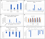
Figure two. Crop producers' profits, consumer surplus and consumer prices nether different scenarios. (A) Change in aggregated ingather producers' profit under different scenarios with reference to the teff export-ban scenario. (B) Regionalized change in aggregated crop producers' profit nether the gratis export scenario—adaptation zone wise. (C) Alter in aggregated crop producers' profit under the costless export scenario—administrative region wise. (D) Changes in aggregated producer, consumer, and consign price of teff under different scenarios. (E) Change in aggregated consumers' surplus under different scenarios with reference to the teff export-ban scenario. (F) Change in aggregated consumers' surplus—administrative region wise for free consign scenario.

Consumer Price of Teff and Revenue From Teff Export

We now evaluate the fluctuations in prices due to changes in export policy, as 1 of the primary reasons to implement a ban on teff export is to curtail increase in the domestic price of teff. We interpret these fluctuations as a direct, first order response to a change in policy, since our model does not include macroeconomic adjustments that might occur in the wake of a change in teff consign policy. Currently, the domestic price of teff averages about 74 U.s.a. dollars (USD) per quintal (Tafere et al., 2010), which is the toll assumed for the base example in simulations. We note that under no restrictions for teff export, our simulations indicate that the price can rise to as high as 91 USD per quintal. This amounts to over a 22% increment in the price of teff. In the model, this has the ability to wipe out teff consumption in certain regions of the state (for example the moist lowlands, adaptation zone M1). This happens because these regions and so have an alternative crop like wheat, barley, or sorghum, which contributes to the utility of the consumer without forcing them to pay significantly higher prices. This substitution has no meaningful impact on the prices of these other grains in our simulations; the change in price of other grains is on the order of 0.05%. Under no taxation for export, the export price is commensurate with the average domestic price. We also note that under the considered milder restrictions on export as opposed to a complete ban, namely a cap of 200,000 quintals or two million quintals of teff export per yr, the price-increase is relatively smaller at 0.58 and 7.5%. Still, if there is an increase in the global demand for teff, fifty-fifty under these milder restrictions on export, increase in domestic prices can be as high as 17 and 18%, respectively. In other words, we observe that the domestic prices of teff could be quite sensitive to global fluctuations of teff demand compared to governmental policies on teff export. The details of these results are shown in Figure 2D. We notation that in each scenario, the decrease in consumer surplus is always exceeded past the increment in producer surplus, past a comparison of Figures 2A,E. Farther, we also see a drop in the consumer surplus for each scenario, and observe that apart from Oromia and Amhara, the desert regions of Somali are significantly affected past the policy change, every bit shown in Figures 2E,F. The simultaneous increase in producer surplus and subtract in consumer surplus in the Oromia and Amhara is explained by the fact that a fraction of self-consumed crops are now exported due to better prices for more than profits, but the decrease in consumer surplus in Somali without an advisable increase in the producer surplus there shows the harmful impact of the policy on the desert region.

Changes in Teff Transport Design and Domestic Consumption

Now we analyze the regions that primarily contribute to teff export and the changes in domestic consumption patterns. Teff from the fertile regions in Amhara and Tigray regions contribute the majority of the teff exported from the country. This is observable in the meaning changes in transportation patterns of teff in Figure 3. We note that the teff that would have otherwise gone to Dire Dawa and thereon to Jijiga and Werder is diverted to Addis Ababa, from where export occurs. We also annotation that relatively small quantities of teff from the Oromia and SNNPR regions of Federal democratic republic of ethiopia are sent for consign.

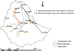
Figure three. Changes in teff transport pattern: The black lines correspond to the connections whose usage decreases after the ban is lifted. The blood-red lines represent to the connections whose usage increases afterwards the ban is lifted. Thickness is proportional to magnitude of alter.

Due to this effect, some markets sell significantly less teff nether the free export scenario than under the baseline instance with the ban in place (Effigy four; note that the pins are scaled to the percentage decrease in quantity sold in the markets). This includes markets in Gondar, Mekelle, Harar and Semera, which are all located in the northern and eastern role of the country. These disruptions are significantly smaller for a scenario of capped exports (Effigy 4). This result suggests that the government'due south proposal to allow regulated quantities of teff export (Abdu, 2015) is less harmful to the local markets and hence consumers than an unregulated teff consign market place. Nonetheless, this still comes at a vulnerability to increase in domestic food prices should there be an upward shift in the global demand bend (e.m., the export + increased demand scenario, Figure 2d).

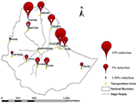
Figure 4. Reduction in quantities sold in domestic markets relative to amount sold under an export ban. Red pin heads correspond to the costless export scenario. White pinheads correspond to the scenario with an export cap of 200 chiliad quintals per year.

Somali, a low fertility arid region of Ethiopia, is the region that is affected the about past the teff export. Information technology is costlier and unattractive for whatever producer to transport teff to Jijiga or Werder than to consign. Thus, these locations suffer a price college than the consign cost of teff. Farther, this leads to decreased consumption of teff in these regions. We exercise note that teff is a smaller portion of local diets in this region compared to many other regions in Ethiopia, so though the impact on teff is substantial the impact on overall diets might not exist overly astringent. At present DECO2 does non account for these sub-national differences in food preference.

Conclusions and Discussions

In this paper,

i. We present the DECO2 model with its more detailed modeling of disaggregation of the food-product regions of Federal democratic republic of ethiopia and,

ii. We use the model to simulate shifts in Ethiopian food markets at regionalized scale in response to changes in teff export policy.

Compared to the fractional equilibrium model presented in Bakker et al. (2018), DECO2 includes a more than detailed representation of food production, using accommodation zones that group regions with similar agro-climatic properties together. DECO2 also has a more sophisticated representation of food markets beyond the country and transport between them, which helps in assessing the distribution of benefits likewise equally quantifying increase in domestic food prices nether a range of regime policies for teff consign. DECO2 is also calibrated based on a more inclusive observational data set from reliable sources.

Discussion of Model Results

We use the status of a complete ban on teff export as the base of operations case. We then use the DECO2 model to identify shifts in equilibrium under scenarios of a completely costless international export market place for teff, and limited consign quantities of 200,000 quintals per yr and two million quintals per twelvemonth. We too run these scenarios nether a constant and then a college global demand for teff.

Nosotros observe that a lion'due south share of the boosted international revenue is enjoyed by the distribution and operating warehouse activities as opposed to the initial production activity, unless the ingather producers are large market actors themselves who as well afford distribution or storage of their produce. Though there is a pocket-sized increment in national revenue during a typical year, a surge in the global demand for teff could cause significant harm to consumers across the state, especially to those in the northern and eastern parts of the country. This also comes with a full general decrease in domestic food consumption under the release of a teff export ban. While these results suggest the lopsided benefits due to removal of teff export ban, nosotros caution confronting interpreting these results as policy prescriptive. A more comprehensive analysis is required to decide if the loss in the welfare of some market actor in some region is outweighed by the benefit for the other. Such assay might require a study based on demographics of the region, potential for intra-land migration, potential for the regime to provide culling benefits and others. Nevertheless, our results are relevant in that they quantitatively equally well as qualitatively capture the impacts of the removal of the ban and can inform discussion of modifications to the ban and relevant complementary policies.

It is likely that in that location are additional policies that may be able to command for the lopsided effects, such as past allowing crop producers to expand into forest and barren lands, improving the usage of irrigation, fertilizers and encouraging better farm management practices, collecting international export taxes, or subsidizing ingather producers given the additional revenue from teff export. These mentioned policies can be modeled past DECO2 with unproblematic modifications, providing ex ante evaluations for the policymakers.

Limitations

While DECO2 has a detailed modeling of spatially explicit food production, transport, and consumption under a partial-equilibrium framework, it has its own set of limitations and simplifying assumptions. Beingness a fractional-equilibrium model, DECO2 assumes invariability of macroeconomic parameters that have pregnant impacts on the variables that are considered in the model. For example, we practice not consider endogenous changes in Gross domestic product of the state throughout the fourth dimension-horizon over which the model is solved. This contrasts with the fact that the Gdp of Federal democratic republic of ethiopia has been growing at about 8–10% per annum over the last decade and might change if the country starts exporting teff. Similarly, Ethiopia has also imported nigh 15 1000000 quintals of wheat per annum in recent years. We again assume that these imports stay constant throughout the time horizon. This assumption of constant imports simplifies interpretation of results, and there is some reason to wait that any large-calibration adjustments in grain imports will be slow relative to the time horizon of our simulations, but making this assumption limits the range of market and policy dynamics at play in our scenarios. The lack of these kinds of adjustments in our model means that results are best interpreted as an estimate of the expected direct impacts of a policy change propagating through the Ethiopian food system, rather than equally a project of a new equilibrium afterward macroeconomic adjustment. It is possible that the straight impacts of a policy alter, as estimated in our simulations, would in fact trigger economic or policy responses that modify the long-term outcomes of the policy.

One can also find differences or changes in preferences of consumers over the class of the simulation period. Changes in social and ecology systems have great implications for the consumption preferences of consumers. Nonetheless, to avert aggregation issues and for ease of calibration we assumed that preferences of consumers remained the aforementioned over the period of analysis. Such an supposition might prevent the states from capturing long-term substitution furnishings in food consumption, but our analysis is over a short time menses over which such dynamics are unlikely to be significant. In addition to the in a higher place listed variables, our model also neglects the presence of any food assistance dependent community, and assumes a constant foreign-exchange rate, fixed interest charge per unit, and a stable political environment (which has implications for transportation).

These assumptions on the macroeconomic variables could be unrealistic if nosotros are interested in future macroeconomic trends. Nonetheless, we observe that the macroeconomic variables impact all the scenarios in a similar way. These macroeconomic variables include imports and exports of all grains. And then, for researchers and policy-makers who are interested in analyzing the direct impacts of policy changes, and evaluating the differences in microeconomic parameters, DECO2 serves as a useful tool to compare policies on a "what-if" basis. If, instead, long-term furnishings of a policy are of interest, it would exist important to capture macroeconomic changes and their sensitivity to simulated policies. This can be accomplished by coupling DECO2 with a computable full general equilibrium model (CGE) or a model that informs DECO2 almost macro-economic changes. In fact, such a coupling between a partial equilibrium model (NANGAM) and a macroeconomic model (GCAM) has been done for free energy markets (Feijoo et al., 2018) and is currently under evolution for DECO2.

Another caveat of the model is that we exercise not consider dual responsibility of any marketplace actor. In reality, information technology is customary in Ethiopia to detect individuals that act every bit both a distributer and owner of a warehouse, or as a producer and a distributer. It is too difficult to disentangle a crop producer from a livestock raiser in some cases, although a sizeable proportion of livestock raisers whose livelihood depends on livestock tin be viewed equally separate from crop producers, particularly in drier adaptation zones. That is why our analysis should exist studied through the lens of regional activities, rather than individuals making decisions. Finally, cattle are traded in Ethiopia as opposed to beef. Withal, since our analysis does not depend upon the supply chain of beefiness, we assume that the livestock raisers slaughter the cattle and sell the final consumable—beef.

The strengths and limitations noted above have to exercise with the structure of the DECO2 model. In add-on, there are caveats associated with the present written report due to data limitations or scenario simplifications that could exist addressed in future work without major changes to DECO2. (i) Nosotros assumed a constant marginal price of farming per area of farmland. Nonetheless, one can model a variable cost through incorporating subcontract investment and direction practices, given available data. (2) We assumed the aforementioned price elasticity for a crop beyond the land; however, in the eastern office of the country teff is not as fundamental to diets, such that cultural preferences could affect regional elasticities. Reliable data about regional differences in toll elasticity can be readily incorporated into DECO2. (3) Nosotros did not consider any cross-price elasticity amongst the dissimilar food items. Market interaction is modeled exclusively by the consumer's objective, in which the market place actor maximizes the sum of utility obtained from all food items. Cross toll elasticity-based marketplace interaction can be incorporated with the availability of relevant reliable data. (4) We practise not account for informal teff export, which is known to occur across some land borders nonetheless the official ban on teff consign, and nosotros exercise not consider the legal catamenia of teff as finished product (i.e., direct export of injera breadstuff). (5) We assume no natural or social barrier that can hinder the crop producers from going to the closest market as adamant past Thiessen polygon overlap with accommodation zone. Consistent data on market preference can be used easily to update the proportion of crop producers going to different markets. (vi) We do not validate the flows in the base case of the model. This is due to lack of reliable data on the quantity of grains transported from 1 region to some other. In the base case, we ensure that the production and consumption at various locations match the data from the key statistical agency and let the model decide the flows. These information are thus synthetically generated, and the best we tin can do with the current scientific discipline and information bachelor to u.s..

Despite the above caveats and limitations, DECO2 serves as a valuable tool to clarify food-related policies based on their impacts at sub-national scale and on diverse groups of market actors in the economy. The model has a regional representation of food product, merchandise, transport, consumption, and export. In this application we have used the model to clarify the regional effects of changes to the teff export policy on different market actors. The resulting scenario analysis can help to identify potential risks and benefits of different approaches to teff export policy, considering both the potential to increase revenue and possible impacts on domestic food grain price and consumption across the country.

Information Availability Statement

All datasets generated for this report are included in the commodity/Supplementary Fabric.

Author Contributions

SSa, YZ, and SSi adult the model equations. SSa programmed the model. YZ programmed and computed the spatial conversion factors and simulated the crop yield model. BE, BS, and BZ provided the relevant food product data for the model. JC analyzed and interpreted the data and helped develop output analysis tools. SSa, YZ, BZ, and SSi designed the sets of scenarios for analysis. SSa, YZ, YN, BZ, and SSi analyzed the results and critically edited the manuscript.

Funding

This piece of work was supported by NSF Grant #1639214 for INFEWS/T1: Understanding multi-calibration resilience options for vulnerable regions.

Conflict of Interest

The authors declare that the research was conducted in the absence of any commercial or financial relationships that could be construed as a potential conflict of interest.

Acknowledgments

We give thanks Molly Brown, University of Maryland, College Park; Kathryn Grace, University of Minnesota and Jeremy Foltz, University of Wisconsin, Madison for their valuable inputs during the study and preparation of this manuscript.

Supplementary Material

The Supplementary Fabric for this commodity can be institute online at: https://www.frontiersin.org/articles/10.3389/fsufs.2020.00004/full#supplementary-material

References

Alem, Y., and Söderbom, M. (2012). Household-level consumption in Urban Ethiopia: the effects of a large food cost shock. World Dev. twoscore, 146–162. doi: x.1016/j.worlddev.2011.04.020

CrossRef Full Text | Google Scholar

Allen, R. Thou., Pereira, L. Southward., Raes, D., and Smith, M. (1998). Crop evapotranspiration-Guidelines for computing crop water requirements. FAO 300:D05109.

Google Scholar

Bakker, C., Zaitchik, B. F., Siddiqui, S., Hobbs, B. F., Broaddus, E., Neff, R. A., et al. (2018). Shocks, seasonality, and disaggregation: modelling food security through the integration of agronomical, transportation, and economic systems. Agric. Syst. 164, 165–184. doi: ten.1016/j.agsy.2018.04.005

CrossRef Full Text | Google Scholar

Bigman, D. (1985). Food Policies and Nutrient Security Under Instability: Modeling and Analysis. Lexington, MA: Lexington Books D.C. Heath and Visitor.

Google Scholar

Central Statistical Agency of Ethiopia (2016). Ethiopia - Demographic and Health Survey. Technical Report, The Federal Democratic Democracy of Ethiopia Central Statistical Bureau, Addis Ababa.

Google Scholar

Fundamental Statistical Bureau of Ethiopia (2015). Area and Production of Major Crops. Technical Report, The Federal Democratic Commonwealth of Ethiopia Key Statistical Agency, Addis Ababa.

Google Scholar

Crymes, A. R. (2015). The International Footprint of Teff: Resurgence of an Ancient Ethiopian Grain. St. Louis, MQ: Washington University.

Google Scholar

Di Falco, S., and Veronesi, M. (2012). How african agriculture can adapt to climate change? - A counterfactual assay from Federal democratic republic of ethiopia. SSRN Electron. J. 89, 743–766. doi: 10.2139/ssrn.2030220

CrossRef Total Text | Google Scholar

Doorenbos, J., and Kassam, A. H. (1979). Yield response to water. Irrig. Drain. Pap. 33, 257–280. doi: 10.1016/B978-0-08-025675-7.50021-two

CrossRef Total Text | Google Scholar

Feijoo, F., Huppmann, D., Sakiyama, L., and Siddiqui, Southward. (2016). N American natural gas model: Impact of cross-border merchandise with Mexico. Energy 112, 1084–1095. doi: 10.1016/j.energy.2016.06.133

CrossRef Full Text | Google Scholar

Feijoo, F., Iyer, G. C., Avraam, C., Siddiqui, S. A., Clarke, L. East., Sankaranarayanan, S., et al. (2018). The hereafter of natural gas infrastructure development in the Usa. Appl. Energy 228, 149–166. doi: ten.1016/j.apenergy.2018.06.037

CrossRef Total Text | Google Scholar

Feijoo, F., Sankaranarayanan, S., Avraam, C., and Siddiqui, S. (2019). Mathematical Models for Evolving Natural Gas Markets. Springer

Google Scholar

Gabriel, S. A., Conejo, A. J., Fuller, J. D., Hobbs, B. F., and Ruiz, C. (2012). Complementarity Modeling in Energy Markets, Springer Scientific discipline and Business Media. New York, NY: Springer Scientific discipline & Business concern Media.

Google Scholar

Getnet, K., Verbeke, W., and Viaene, J. (2005). Modeling spatial cost transmission in the grain markets of Ethiopia with an application of ARDL approach to white teff. Agric. Econ. 33, 491–502. doi: x.1111/j.1574-0864.2005.00469.x

CrossRef Full Text | Google Scholar

Gilbert, C. L. (2012). International agreements to manage nutrient price volatility. Glob. Food Sec. one, 134–142. doi: 10.1016/j.gfs.2012.10.001

CrossRef Total Text | Google Scholar

Iizumi, T., Luo, J.-J., Challinor, A. J., Sakurai, Grand., Yokozawa, Chiliad., Sakuma, H., et al. (2014). Impacts of El Niño Southern Oscillation on the global yields of major crops. Nat. Commun. v:ncomms4712. doi: ten.1038/ncomms4712

PubMed Abstract | CrossRef Full Text | Google Scholar

Jaleta, Thou., and Gebremedhin, B. (2012). Price co-integration analyses of food crop markets: the case of wheat and teff commodities in Northern Ethiopia. African J. Agric. Res. vii, 3643–3652. doi: ten.5897/AJAR11.827

CrossRef Full Text | Google Scholar

Kumar, N., and Quisumbing, A. R. (2013). Gendered impacts of the 2007–2008 nutrient cost crunch: evidence using panel data from rural Ethiopia. Food Policy 38, eleven–22. doi: ten.1016/j.foodpol.2012.ten.002

CrossRef Full Text | Google Scholar

Mccornick, P. One thousand., Awulachew, Southward. B., and Abebe, M. (2008). Water –food –energy –environment synergies and tradeoffs: major issues and case studies. Water Policy i, 23–26. doi: 10.2166/wp.2008.050

CrossRef Full Text | Google Scholar

Minten, B., Taffesse, A. Due south., and Brown, P. (2018). The Economics of Teff: Exploring Federal democratic republic of ethiopia's Biggest Greenbacks Ingather. Washington, DC: International Nutrient Policy Enquiry Institute (IFPRI).

Google Scholar

Negassa, A., and Jayne, T. S. (1997). "The response of ethiopian grain markets to liberalization," Working Paper No. vi (Addis Ababa: Grain Market Research Project).

Google Scholar

Provost, C., and Jobson, East. (2014). Move over Quinoa, Ethiopia's Teff poised to be next big super grain. Guardian.

Google Scholar

Robinson, South., Stonemason-D'Croz, D., Sulser, T., Islam, S., Robertson, R., Zhu, T., et al. (2015). The International Model for Policy Analysis of Agricultural Commodities and Trade (Touch on): model description for Version 3. SSRN Electron. J. doi: 10.2139/ssrn.2741234

CrossRef Full Text | Google Scholar

Rosegrant, 1000. Due west., Msangi, S., Ringler, C., Sulser, T. B., Zhu, T., and Cline, S. A. (2008). International Model for Policy Assay of Agricultural Commodities and Trade (Touch): Model description. Washington, DC: International Food Policy Enquiry Institute.

Google Scholar

Sankaranarayanan, S., Feijoo, F., and Siddiqui, S. (2018). Sensitivity and covariance in stochastic complementarity problems with an awarding to N American natural gas markets. Eur. J. Oper. Res. 268, 25–36. doi: 10.1016/j.ejor.2017.xi.003

CrossRef Total Text | Google Scholar

Sethi, S., and Sorger, G. (1991). A theory of rolling horizon decision making. Ann. Oper. Res. 29, 387–415. doi: 10.1007/BF02283607

CrossRef Full Text | Google Scholar

Sharma, R. (2011). "Food export restrictions: review of the 2007-2010 experience and considerations for disciplining restrictive measures," Working Paper No. 32 (Rome: FAO Commodity and Merchandise Policy).

Google Scholar

Tafere, M., Taffesse, A. South., Tamru, Due south., Tamiru, S., Tefera, Due north., and Paulos, Z. (2010). "Food need elasticities in Federal democratic republic of ethiopia: estimates using Household Income Consumption Expenditure (HICE) survey information," ESSP Working Papers 11 (Washington, DC: International Food Policy Research Institute (IFPRI)).

Google Scholar

Tamru, S. (2013). "Spatial integration of cereal markets in Federal democratic republic of ethiopia," in Ethiopia Strategy Support Program-Ethiopian Evolution Research Institute (Washington, DC).

Google Scholar

USDA Foreign Agronomical Service (2013). Ethiopia Grain and Feed Almanac.

Google Scholar

Voronoi, M. M. (1908). Nouvelles applications des param'etres continus 'a la th'eorie des formes quadratiques. deuxi'eme M'emoire: Recherches sur les parall'ello'edres primitifs. J. Reine Angew. Math. 134, 198–287. doi: ten.1515/crll.1908.134.198

CrossRef Full Text | Google Scholar

Wailes, E. J., and Chavez, E. C. (2011). "2011 Updated Arkansas Global Rice Model," in Staff Paper 1. Fayetteville, AR: University of Arkansas, Department of Agricultural Economics & Agribusiness, Division of Agronomics.

Google Scholar

Woldie, Chiliad. A., and Siddig, Chiliad. (2009). The Affect of Banning Export of Cecreals in Response to Soaring Food Prices: Testify From Ethiopia Using the New GTAP African Database. Giessen: Munich Papers. RePEc Curvation.

Google Scholar

Wossen, T., Di Falco, S., Berger, T., and McClain, Westward. (2016). You lot are not alone: social capital and take a chance exposure in rural Ethiopia. Nutrient Secur. 8, 799–813. doi: x.1007/s12571-016-0587-five

CrossRef Full Text | Google Scholar

dylandundas.blogspot.com

Source: https://www.frontiersin.org/articles/10.3389/fsufs.2020.00004/full

Berbagi :